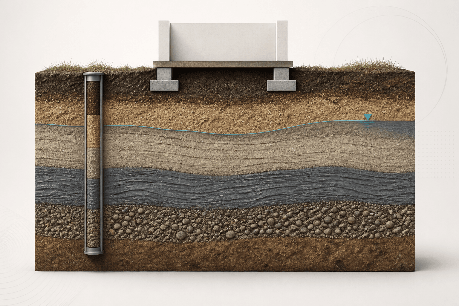
After this chapter, you should be able to
- Distinguish settlement mechanisms and timescales.
- Interpret e–log stress behaviour and stress history.
- Calculate a normally consolidated layer settlement.
- Estimate consolidation time using a stated drainage path.
- Identify when a one-dimensional estimate is insufficient.
Engineering context and evidenceSource §Lesson 05 · Engineering context and evidence · NHI-06-088 Chapters 5 and 7
Settlement is a compatibility and serviceability problem as much as a vertical displacement calculation. Immediate distortion, primary consolidation and secondary compression may occur in different proportions and at different rates. The engineer must define the loading sequence, drainage boundaries, stress history and spatial variability before selecting a method.
Core principles and terminologySource §Lesson 05 · Core principles and terminology · NHI-06-088 Chapters 5 and 7
In saturated fine-grained soil, an applied stress may initially raise pore pressure. Drainage transfers stress to the soil skeleton and volume reduces with time. Oedometer data idealize one-dimensional strain; sample disturbance and selection of preconsolidation stress, compression index and coefficient of consolidation can dominate the result.
- Compression index, Cc
- Slope parameter for the virgin compression portion of an e–log10 σ′ curve under the adopted convention.
- Preconsolidation stress
- Interpreted maximum past effective stress or equivalent yield stress in the one-dimensional model.
- Coefficient of consolidation, cv
- Parameter controlling the rate of one-dimensional consolidation for stated test conditions.
- Drainage path, Hdr
- Maximum distance pore water travels to a drainage boundary in the idealized layer.
Equations, conventions and valid useSource §Lesson 05 · Equations, conventions and valid use · NHI-06-088 Chapters 5 and 7
This teaching form assumes a representative normally consolidated layer and one-dimensional strain. Subdivide layers and use recompression/virgin branches where stress history requires them.
Select Tv for the required average degree of consolidation using the adopted solution. Hdr is H/2 only when both boundaries drain.
Engineering workflowSource §Lesson 05 · Engineering workflow · NHI-06-088 Chapters 5 and 7
- Define foundation loads, excavation, fill placement and construction sequence.
- Build initial effective-stress and stress-increase profiles through compressible strata.
- Separate immediate, primary and secondary mechanisms.
- Review sample quality and interpret e0, preconsolidation stress, Cc/Cr and cv by layer.
- Subdivide thick or variable layers and integrate settlement contributions.
- Select single- or double-drainage paths from actual boundaries, not from habit.
- Compare total and differential settlement with structural tolerance and observational controls.
| Mechanism | Typical evidence | Key uncertainty |
|---|---|---|
| Immediate | Stiffness and stress distribution | Strain level and anisotropy |
| Primary consolidation | Oedometer compression and cv | Stress history and drainage |
| Secondary compression | Long-duration test response | Time origin and structure |
| Differential settlement | Spatial ground/load model | Variability and structural interaction |
Verified teaching exampleSource §Lesson 05 · Verified teaching example · NHI-06-088 Chapters 5 and 7
Normally consolidated layer estimate
A 3.0 m layer has e0 = 0.90, Cc = 0.30 and initial σ′0 = 100 kPa. Loading adds 80 kPa. For a 90% average-consolidation rate illustration use cv = 2.0×10⁻⁸ m2/s, Hdr = 1.5 m and Tv = 0.848.
- Final stress
σ′f = 100 + 80
σ′f = 180 kPa - Settlement
Sc = 3×0.30/1.90×log10(180/100)
Sc = 0.121 m - Illustrative 90% time
t90 = 0.848×1.52/(2.0×10−8)
t90 = 9.54×10⁷ s ≈ 1104 days ≈ 3.02 years
Result. The idealized primary settlement is about 121 mm and the FHWA tabulated Tv = 0.848 state for 90% average consolidation is reached in about 3.02 years. Both results are highly sensitive to the layer model and parameters.
One-dimensional consolidation teaching check
Reproduce the stated normally consolidated settlement and time-factor equations.
- Inputs
- H, e0 and Cc · Initial effective stress and stress increase · cv, Hdr and Tv
- Outputs
- Primary consolidation settlement · Final effective stress · Illustrative time in seconds, days and years
- Status states
- Complete teaching case · Invalid or non-finite input · Outside stated method domain
- Validation
- Implemented against the supplied worked example; independent technical approval pending
One-Dimensional Consolidation Settlement
A narrow normally consolidated layer calculation using log10 stress and a separately stated time factor.
Idealized primary settlement is 120.9 mm; the selected Tv state occurs at 3.02 years.
- Final effective stress σ′f
- 180.00 kPa
- Primary settlement Sc
- 0.1209 m (120.9 mm)
- Time t
- 9.540e+7 s
- Time
- 1104.2 days (3.02 years)
Show calculation trail
σ′f = σ′0+Δσ′ = 180.00 kPaSc = H Cc/(1+e0) log10(σ′f/σ′0) = 0.1209 mt = Tv Hdr2/cv = 9.540e+7 s
Failure modes and engineering judgementSource §Lesson 05 · Failure modes and engineering judgement · NHI-06-088 Chapters 5 and 7
- Using total stress where the compression model requires effective stress.
- Applying the virgin compression line below preconsolidation stress.
- Assuming double drainage without a permeable boundary.
- Using one oedometer result for a heterogeneous deposit.
- Checking only total settlement and ignoring differential movement and angular distortion.
Key points
- Settlement mechanisms and time must be separated before calculation.
- Stress history and sample quality strongly influence parameters.
- Drainage path is a physical boundary condition, not a default.
- Differential movement and construction sequence often control serviceability.
Source references recorded by the supplied chapter
- FHWA NHI-06-088, Soils and Foundations Reference Manual, Volume I, Chapters 5 and 7.